Cool Mathematics

e Day (e) February 7 (2-7)	e = 2.7 1828 1828 4590…
Pi Day (π) March 14, 2016 (3-14-16)	π = 3.14 159 265 358 979 …
Phi (φ) Jan 6, 2018 (1-6-18)	φ = 1.618 033 988 750 …

"Mathematics is the alphabet with which God has written the Universe."
— Galileo Galilei

Cool Math History

al-jabr

A lgebra is from the Persian, al-jabr (reunion, restoration), from the book, Hibab al-jabr wal-muqubala (Book of Reunion & Balancing), written in 825 in Baghdad, by the Persian Polymath, Muhammad ibn Mūsā al-Khwārizmī (780-850), aka The Inventor of Algebra. His book was translated into Latin as Algoritimi de numero Indorum.

He was the first to use zero as a placeholder for the Hindu-Arabic Numerals.
He was the first to present solutions for Linear and Quadratic equations
From the Latin translation comes Algorithm (the logical steps for solving a problem)

Algebrista

T he word al-jabr was used by the Moors of Spain who were of Persian descent. To the Moors, an Algebrista was a Bonesetter, or "restorer" of bones. Throughout Europe during medieval times, a Barber (from the Latin 'barba', beard) were also known as an Algebrista, since they often did bone-setting, bloodletting, and tooth extraction on the side. This led to the Traditional RED and WHITE (Blood & Bone) striped Barber poles in front of Barber shops. At the base of the pole was a Brass Basin for collecting blood.

B arbering began in Rome circa 300 B.C. with all Free Men required to be clean-shaven, while slaves were forced to wear beards. Alexander the Great demanded that all of his forces be clean-shaven as an advantage in hand-to-hand fighting.

W hen spinning, the RED stripes on Barber Poles give the impression of blood flowing down to fill the basin. When NOT spinning, the RED stripes represented the bloody bandages wrapped around a patient's arm. (In the U.S. a BLUE stripe has been added to match patriotic colors)

💈 A Classic Red/White Barber Pole

T rigonometry is from the Greek, trigónon (triangle) and metron (measure). Although some of the concepts were used as long ago as when the pyramids were built in ancient Eqypt, the field emerged with a renewed vigor during the 3rd and 4th centuries from studies related to astronomy.

C alculus, from the Latin, calculus (pebble, counter), was created and developed in the 17th century by Sir Isaac Newton (1642-1726) and independently by Gottfried Wilhelm Leibniz (1646-1716) as a tool to better explain the Laws of Gravitation and Motion. In 1687 Sir Isaac Newton published his famous book, Philosophia Naturalis Principia Mathematics, which laid the foundation for all clasical mechanics.

O f special mention is Leonardo Fibonacci (1170-1250), an Italian Mathematician (a.k.a. Leonardo of Pisa). He published a book in 1202 entitled Liber Abaci (Book of Calculation) which introduced Europe to Fibonacci Numbers & the Golden Ratio. He is credited with being the first to introduce Europe to the Hindu-Arabic decimal number system. Many consider him to be the most talented Western Mathematician of the middle ages.

The Golden Ratio, Phi (φ)

φ - 1 =

φ = 1.6180339887…
1/φ = .6180339887…

φ =

1 + √5

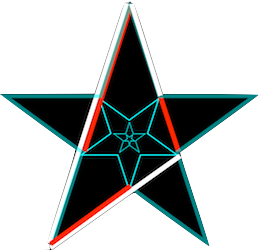
Golden Rectangles create a Golden Spiral

The Pentagram Contains Many Golden Ratios (φ)
It can re-create itself indefinitely! ☞ ☞ ☞ ☞ ☞

A knot tied with paper will ALWAYS generate a pentagon.

Let Red = 1
then White = φ (1.6180339887…)

The Fibonacci Series → Golden Ratio (φ)

Pick ANY two numbers, NOT BOTH ZERO. (fractional, big, small, negative, whatever)
Create a Fibonacci Series by simply adding together the preceding two numbers to create the next.

Clasic Fibonacci Series: 0, 1, 1, 2, 3, 5, 8, 13, 21, 34, 55, …
A Random Fibonacci Series: -1.5, 16, 14.5, 30.5, 45, 70.5, 120.5, 191, 311.5, …

The RATIO of any term in the series to the previous term approaches the Golden Ratio (φ).

Lim_n→∞ X_n ⁄ X_n-1 = φ

Trigonometry

The Setup

First we draw a horizontal line ONE unit long.
The line's left side endponit will be the Origin. As the line sweeps around counter-clockwise from this origin, it describes a circle of Radius = 1 and Circumference = 2π.
As the line sweeps it describes an angle θ measured from the original horizontal line.

The Definitions

Each angle α describes a right triangle whose hypotenuse, C = 1.
The vertical line A = sin(α)
The horizontal line B = cos(α)
The ratio of the sin to the cos is the tangent. tan(α) = ^A ⁄ _B

A² + B² = C²

The Pythagorean Theorem

Double Angle Formulas
sin (2A) = 2 sin A · cos A
cos (2A) = cos²(A) - sin²(A)

As the angle α, increases past 2π Radians (360°)
sin and cos cycle between -1 and 1
and graph as a sine wave…

A wheel spinning along a straight path
also generates a sine wave.
This is known as Simple Harmonic Motion…

Trigonometric Algebra

sin(α + β) = sin(α)·cos(β) ± cos(α)·sin(β)
cos(α + β) = cos(α)·cos(β) ∓ sin(α)·sin(β)

Trigonometric Series
Gottfried Wilhelm Leibniz developed these Series Formulae for Sine and Cosine
(x in radians) (! is factorial, e.g. 5! = 5 x 4 x 3 x 2 x 1)

sin x = x - (x³ ⁄_3!) + (x⁵ ⁄_5!) - (x⁷ ⁄_7!) + …

cos x = 1 - (x² ⁄_2!) + (x⁴ ⁄_4!) - (x⁶ ⁄_6!) + …

Calculus

Differentiation (Tangent Slope)

The Derivative of a function is defined as the Tangent Slope at each x of the function ƒ(x)
and is written as:

^d⁄_dx ƒ(x)

(the derivative, with respect to x, of the function of x)

A shorthand notation is:

ƒ′ (x)

(f prime of x)

^d⁄_dx xⁿ = n x^(n-1) ^d⁄_dx e^x = e^x

^d⁄_dx sin(x) = cos(x) ^d⁄_dx cos(x) = - sin(x)

Partial Differentiation (∂)
For functions with multiple variables (x, y, z, t, …), the Partial Derivative is defined as the
Derivative of the function with all variables EXCEPT ONE held constant. It is written as:

^∂⁄_∂t ƒ(x, y, z, t …)

(the partial derivative, with respect to t, of the function of x, y, z, t etc.)

Integrals (Sum of Areas Under Curve)

The Integral of a function is defined as the Sum of the Areas between the function and the x-axis, written as:

∫ ƒ(x) dx

(the integral of the function of x with respect to x)

A Definite Integral of a function is the Sum of the Areas between the function and the x-axis
Only between x=a and x=b, written as:

_a ∫^bƒ(x) dx

(the integral, from a to b, of the function of x with respect to x

Some examples (n ≠ -1) …

∫ axⁿ dx = ax⁽ⁿ⁺¹⁾ ⁄ (n+1) + C

∫ ¹⁄_x dx = ln |x| + C

∫ e^x dx = e^x + C

∫ x² dx = ^x³⁄₃ + C

∫ sin(x) dx = -cos(x) + C

∫ cos(x) dx = sin(x) + C

The Bell Curve

S tatistical Analysis makes use of families of distribution curves which are known as Bell Curves. Here is one.

φ(x) = ke ^{(- π x²)}

Where
k = height of the Bell Curve

The Amazing Ellipse

1 =

x²

a²

y²

b²

An ellipse can be defined from two fixed foci F₁ , F₂ using a given constant length L where:

L = (F₁, P) + (P, F₂)

Matrix Mathematics

A Matrix is a grouping of data elements arranged in rows and columns.
The elements can represent numbers, expressions, or any type of data.
Matrices are 'built' column by column
Matrices are named as: Rows x Columns, e.g. A[3x2] , B[2x3]
Subscripts are used to identify Matrix elements (Row, then Column)

N_{row, column}

Matrix Multiplication

Matrix Multiplication is NOT cummutative. A x B ≠ B x A
The number of columns in the 1st must equal the number of rows in the 2nd.

Example: A[3x2] x B[2x3] = C[3x3]

(A_1,1 · B_1,1) + (A_1,2 · B_2,1) = C_1,1
(A_1,1 · B_1,2) + (A_1,2 · B_2,2) = C_1,2
(A_1,1 · B_1,3) + (A_1,2 · B_2,3) = C_1,3

(A_2,1 · B_1,1) + (A_2,2 · B_2,1) = C_2,1
(A_2,1 · B_1,2) + (A_1,2 · B_2,2) = C_2,2
(A_2,1 · B_1,3) + (A_2,2 · B_2,3) = C_2,3

(A_3,1 · B_1,1) + (A_3,2 · B_2,1) = C_3,1
(A_3,1 · B_1,2) + (A_3,2 · B_2,2) = C_3,2
(A_3,1 · B_1,3) + (A_3,2 · B_2,3) = C_3,3

Matrix Addition , Subtraction

Matrices must be identical in size.

A_1,1

A_1,2

A_2,1

A_2,2

B_1,1

B_1,2

B_2,1

B_2,2

C_1,1

C_1,2

C_2,1

C_2,2

A_1,1 + B_1,1 = C_1,1
A_2,1 + B_2,1 = C_2,1

A_1,2 + B_1,2 = C_1,2
A_2,2 + B_2,2 = C_2,2

Complex Numbers

A Complex Number z is a combination of a Real Number and an 'Imaginary' Number, where
i is defined as √-1 and i ² = -1

z = a + bi

Its Conjugate z is its reflection along the Real Number axis, so:

z = a — bi

The Absolute Value |x| of any number is defined as its Distance from the Origin, Therefore

|z| = √ a² + b²

From this it follows that:

|z|² = z z

Why do we use Imaginary Numbers?

All n-degree polynomials with real coefficients will then have n roots, making algebra " complete. "

It is interesting to note that zero and negative numbers were for centuries viewed as 'make-believe' too.

Curves of Constant Width

The Hohmann Transfer Orbit

Δ V = Δ v₁ + Δ v₂

T he process is 100% reversible, i.e. it can be used to go from a Lower Orbit to a Higher Orbit or from a Higher Orbit to a Lower Orbit.

v_o = √

G M

v_o = Orbital Velocity
r = radius of orbit

Δ v₁ = √

G M

R₁

( √

2 R₂

R₁ + R₂

- 1 )

Δ v₁ = Change in Velocity to enter Ellipse

Δ v₂ = √

G M

R₂

( 1 - √

2 R₁

R₁ + R₂

)

Δ v₂ = Change in Velocity to enter Orbit 2

Reference

Perigee = the nearest point from a Center of Mass in an orbit
Apogee = the farthest point from a Center of Mass in an orbit

Geostationary Orbit ~ The Orbital Velocity matches Earth's Rotional Velocity and is aligned directly over the Equator. These are always circular orbits at 35,786 km (22,236 mi) above the Earth's Equator and rotating in the same direction as Earth. The value R (distance from center of planet) = 42,164 km (26,200 mi).

GPS (Global Positioning System) Orbits are usually Geostationary Orbits. In order for them to be useful and accurate the signals sent and received MUST take into account the relativistic effects of the Speed of Light in a Gravitational Field.

Geosynchronous Orbit ~ The Orbital Velocity matches Earth's Rotional Velocity but these orbits are inclined to the Equator and can be quite elliptical.

Polar Orbits are Low Earth Orbits circling from pole to pole in about 1.5 hours. In 1 day they can see all of the Earth's surface as it rotates below. They are very useful for monitoring changes in the Earth's environment.

1 Earth Rotation, a.k.a. 1 Sidereal Day = 23 hours, 56 minutes, 4.09 seconds OR 23.93447 hours

The Escape Velocity at a given height is √2 times the velocity in a circular orbit at the same height.

Gravitational Assist (Fly By)

f ⁄ stops

The first ten Standard ƒ/stop numbers are calculated thus...

ƒ/ (√ 2 )⁰ ƒ/ (√ 2 )¹ ƒ/ (√ 2 )² ƒ/ (√ 2 )³ ƒ/ (√ 2 )⁴ ƒ/ (√ 2 )⁵ ƒ/ (√ 2 )⁶ ƒ/ (√ 2 )⁷ ƒ/ (√ 2 )⁸ ƒ/ (√ 2 )⁹

Which are approximated to these accepted values...

ƒ ⁄ 1 ƒ ⁄ 1.4 ƒ ⁄ 2 ƒ ⁄ 2.8 ƒ ⁄ 4 ƒ ⁄ 5.6 ƒ ⁄ 8 ƒ ⁄ 11 ƒ ⁄ 16 ƒ ⁄ 22

Why √ 2 ?

The Area of a circle (aperture) = π r²

Each higher ƒ ⁄ stop (n) is half the Area of the previous, so:

1) π r_n+1² = π r_n² ⁄ 2

2) r_n+1² = r_n² ⁄ 2

3) r_n+1 = r_n ⁄ √ 2

The Tesla Vortex 3-6-9

Ocean Waves

hen the water depth becomes less than one-half the wavelength (D < L ⁄ 2), the deep-water swell begins to 'feel' the ocean floor. The drag on the water caused by the ocean floor begins to slow down the wave. The wavelength (L) shortens and its height (H) increases. The trough of the wave slows down and the top begins Peaking. Eventually the Peak overtakes the the slower bottom of the wave until a point is reached when the wave becomes unstable. The Peak spills over and the wave becomes turbulent. The wave has become a Breaker.

ir can become trapped within the Curl of the Breaker and will sometimes explode out a side of the Breaker (common in Point Breaks), or the top of the Breaker (common in Shore Breaks).

eep water waves (D >> L ⁄ 2) will also sometimes break, forming White Caps, when the surface wind increases the wave height to a point where the Peak angle falls below 120°, corresponding to a wave height ratio of H = L ⁄ 7 . This usually occurs when surface winds reach 8-10 knots (9-12 mph).

ogue waves aren't only freak big waves. They can also manifest as extra-deep troughs, or holes, into which a ship can fall and possibly be overwhelmed by the next wave crest. Statistical analysis predicts that one wave in 23 is over 2x the average height, and one in 1,175 is over 3x the average height, but only one in 300,000 may exceed 4x the average height.

Break

The wave height is greater than one-seventh of the wavelength (H > L ⁄ 7 )
The crest of the wave forms an angle less than 120°

1 Knot = 1 Nautical Mile per Hour
1 Nautical Mile = 1 Minute of Latitude

TSUNAMI WAVES

Since Tsunami waves have very long wavelengths (100 - 1,000 km) and very long periods (1hr or more), they should be considered as shallow-water waves, even in the deepest oceans.

TIDES

A tide is the longest wave on Earth, having a wave length that is half the circumference of the earth and a period of 43,000 seconds (12 hr, 25 min).

Fluid Dynamics

The Boundary Layer

ny viscous fluid traveling past a smooth surface creates a Boundary Layer whose thickness in the Y direction, and Drag on the surface, are a function of the Reynold's Number (Re) (below). The relative velocity exactly at the surface always remains zero (U_x = 0). What starts as Laminar Flow (L, where Drag occurs, Re < 1000) quickly transistions (Δ) into a region of Turbulent Flow (T, where Drag approaches zero, Re > 1500).

ipe flows create Internal Boundary Layers (one from each side) that meet in the pipe's center and transistion into only Turbulent Flow in the pipe. For Pipes then, Laminar Flow occurs when Re < 2000 and Turbulent Flow occurs when Re > 4000. In a similar fashion, air rushing into an intake on an airplane engine will experience Turbulent Flow that must be reckoned with at supersonic speeds (Mach 1+).

Flow Regions U(t)

olf balls are 'dimpled' to create Turbulent flow when in flight, reducing drag and improving their flight distance considerably. In the 'Old Days' of Baseball, some pitchers illegally hid sandpaper in their gloves to roughen-up new baseballs so as to improve their fast ball speeds.

merica's Cup racing sailboats are forbidden to 'dimple' their hulls in order to improve their speed and thus gain an unfair advantage over smooth hulls. Seawater is roughly 800 times denser than air so any reduction in Drag can be a significant factor in a race.

he Reynold's Number (Re ) MUST be maintained whenever modeling flows such as for boats or aircraft.

The viscosity of a fluid is a measure of its resistance to deformation over time — i.e. how thick it seems & how fast it will flow. It is given the Greek symbol mu (μ), and quantifies the internal frictional forces between adjacent layers in any fluid (water, oil, air). For instance, maple syrup has a high viscosity, alcohol has a very low viscosity. Glass, which is considered not a solid but a Super-Cooled Liquid, also has viscosity and will flow and deform over extended periods of time. Windows in centuries-old Cathedrals in Europe, bear this out. Their lower sections of glass are now thicker than the top sections. Even Granite Rock has viscosity, although many orders of magnitude above most materials considered fluid.

iscosity of any fluid will change as a function of Temperature. This property is addressed in Motor Oil labels, which are given two viscosity numbers, one for cold and one for hot engines. e.g. 0w-20, 10w-40, etc.

Viscosity Comparisons

Material	10^-3 Pa·s *
Air	0.0018
CO₂	0.0015
Water	1.0
Ethanol	1.1
Mercury Hg	1.5
Blood	3 - 4
Olive Oil	56
Granite	5 x 10¹⁹ Pa·s

* 1 Pa·s = 1 kg /m /s

Logrithms & Exponents

a = 10^{(log₁₀ a)}

a = e^{(ln a)}

a ^b = e^{(b · ln a)}

a ^b· a ^c = a^{(b + c)}

a^(p/q) = q√ a ^p

log_n (a·b) = log_n(a) + log_n(b)

Logarithms and Exponents are symmetrical about y = x

n ⁰ = 1
log_n 1 = 0

Example:
5 ³ = e ^{(3 · ln 5)} = 125

Slide Rules

T he Slide Rule was invented by William Oughtred in 1622. They are accurate to 3 significant places, need no batteries, and were on many manned space missions as a reliable backup calculator.

Slide Rules compare Logrithmic Scales that slide past each other.
To multiply a·b, compare the C & D Scales:

log(a) + log(b) = log(a · b)
[D scale] + [C Scale] = [D Scale]

K Scale = 3 log Scales → x³ Cubes & Cube Roots (from the D Scale)

A Scale = 2 log Scales → x² Squares & Square Roots (from the D Scale)

B Scale = 2 log Scales → x² Squares & Square Roots (from the C Scale)

T Scale = Tangents (from the D Scale, in Degrees)

S Scale = Sines (from the D Scale, in Degrees)

CI Scale = Inverse of C Scale → 1/x (from the C Scale)

C, D Scales = 1 log Scale → Multiplication, Division

Loan Amortization

A = P

i(1 + i)ⁿ

(1 + i)ⁿ - 1

A = periodic payment amount
P = amount of principal
i = periodic interest rate (APR÷12 for monthly)
n = total number of payments

Using a Spreadsheet PMT Function

The spreadsheet will use four cells (A, P, i, n)
- A Payment amount per period (the answer will show here)
- P Enter the Loan Amount
- i Enter the Periodic Interest Rate (monthly = APR ÷ 12)
- n Enter the Number of Payments (e.g. 5 years = 60)
Click in the blank A cell, type: "=-pmt" (equals, minus, "pmt"), then "ENTER"
Click on PMT, the formula will expand...
Systematically select the appropriate cell for each of the first 3 terms
ENTER
DONE! You have your fully amortized Payment amount A

Adjusting the amounts in P, i, n will update the Payment amount A.

Cool Equations

γ =

√

( 1 -

v²

c²

)

1905 Lorentz Transform

λ =

√

( 1 -

v²

c²

)

λ =

√

( 1 -

v²

c²

)

1924 Louis de Broglie Equation

F = G

M₁ M₂

r²

1686 Newton's Law of Universal Attraction

v_o = √

G M

Orbital Velocity
r = distance of object to center of Mass

v_e = √

2 G M

Escape Velocity
R = Radius of solid celestial object

γ = 1 ⁄ √1- (v² ⁄ c²)

γ =

√1 - (v² ⁄ c²)

Lorentz Transforms - Compact

e = hv

e = mc²

1905 Einstein Equation

i ħ ^∂⁄_∂tΨ = Ĥ Ψ

1925 Shrödinger Equation

Δx Δp ≥

ℏ

1927 Heisenberg Uncertainty Principle

⟮ βm ² + c ⟮ ∑ n=1 3 α_np_n ⟯ ⟯ Ψ (x,t) = i ℏ

Circle r = radius	r² = x² + y²
Ellipse a = width, b = height	1 = x² a² + y² b²
Parabola	y = x²
Hyperbola	y = 1 x

1928 Dirac Equation
γ^μ ( 𝑖∂_μ - eA_μ ) 𝛹 = m𝛹

( 𝑖∂⃒ - 𝑚) 𝛹 = 𝛰

Dirac Equation re-written using Planck Units (ℏ = c = 1)

as Δt → 0 E → photon + e^- + e⁺ → E

1955 Wheeler's Quantum Foam

Re =
ρvL
———
μ
=
vL
———
ν

Reynold's Number

Φ(x) = ke ^{(- π x²)}

Distribution (Bell) Curves

r = sin (nθ) + n

1924 Louis de Broglie Electron Orbitals
sin x = x —

x³

3!
+

x⁵

5!
—

x⁷

7!
+ …
cos x = 1 —

x²

2!
+

x⁴

4!
—

x⁶

6!
+ …
Transcendental Series Definitions

π = Σ n = 0 ∞

4 (-1)ⁿ

2n + 1

π = 4 —

4

3
+

4

5
—

4

7
+

4

9
— …
π Infinte Series
Nilakantha Somayaji (c 1500), James Gregory (1671), & Gottfried Leibnitz (1674)

π = Σ n = 0 ∞

(5n + 3)n!(2n)!

2^n-1(3n + 2)!

π Infinte Accelerated Series ~ Nilakantha Somayaji (c 1500)

e^{π i} = -1
e^xi = cos(x) + i·sin(x)

Euler's Formula

e = Lim n → ∞ (1 +
1
n
)ⁿ

Euler's Number
sin(α + β) = sin(α)·cos(β) ± cos(α)·sin(β)
cos(α + β) = cos(α)·cos(β) ∓ sin(α)·sin(β)

Transcendental Algebra
ax² + bx + c = 0
Quadratic Equation
x = -b ± √b² - 4ac
2a
Quadratic Equation Solution, a ≠ 0

_a∫^b ƒ(x) dx

_n=1∫^∞ ƒ(x) dx

Definite Integrals

∫ axⁿ dx =
ax⁽ⁿ⁺¹⁾
n + 1
+ C

Indefinite Integrals

R_s =
2GM
c²

Schwarzschild Radius for Black Holes

R =

2πc²h

λ⁵ ( e ^{(hc ⁄ λkT)} - 1)

R = Radiant Energy Density as a function of Wavelength λ & Temperature T in °K
c = Speed of light
h = Planck's constant
k = Boltzmann constant
e = Euler's number

Planck's Law of Blackbody Radiation

ƒ(x) =

5.932264822·10^-17

x⁵ ( e ^{(1.74797·10^-5 ⁄ nx)} - 1)

n varies the height of the curve, (0 < n ≤ 1)
Planck's Law of Blackbody Radiation (for graphing purposes)

Circle
r = radius r² = x² + y²

Ellipse
a = width, b = height 1 =
x²
a²
+
y²
b²

Parabola y = x²

Hyperbola y =
1
x

The Conic Sections

Mathematics Limerick

12 + 144 + 20 + 3√ 4

+ ( 5 x 11 ) = 9² + 0

A dozen, a gross, and a score,
Plus three times the square root of four
Divided by seven
Plus five times eleven
Is nine squared and not a bit more.

Roman Numerals

Ⅰ	Ⅴ	Ⅹ	Ⅼ	Ⅽ	Ⅾ	Ⅿ
1	5	10	50	100	500	1,000
	Ⅴ	Ⅹ	Ⅼ	Ⅽ	Ⅾ	Ⅿ
	5,000	10,000	50,000	100,000	500,000	1 million

First used in ancient Rome circa 800 B.C. Modern use is mainly Artistic.
Vinculum ( ) - In Mathematics, a line placed over a group of Mathematical symbols or expressions to be considered as a group. In Roman Numerals the Vinculum multiplies the Roman Numeral by 1,000.

Basic Rules of use:
1. ADD from Left to Right, largest Roman Numerals first.
2. All smaller numerals LEFT of a larger numeral SUBTRACT from the larger numeral
3. Never repeat more than 3 of any Numeral.
4. Ⅴ, Ⅼ, Ⅾ, Ⅴ, Ⅼ, and Ⅾ are never repeated.

EXAMPLES
4 IV NOT IIII
6 VI
9 IX NOT VIIII
12 XII
400 CD NOT CCCC
1776 MDCCLXXVI
1950 MCML
1999 MCMXCIX
2024 MMXXIV

A Few Modern Uses...

Clock Faces / Sundials
Movie & TV year of production
A $100 bill is called a C Note
Outline Lists
Building cornerstones
Monument dates
Water depths on bridge columns
Gravestones
Monarch first names (Louis XIV)
Book prefaces page numbers
Art Deco (V replaces U)

The Best Number is 73

7 x 3 = 21 and 73 happens to be the 21^st PRIME number
7 and 3 are also PRIMES
The mirror of 73 is 37 which is the 12^th PRIME number (and 12 is the mirror of 21)
The number written out, Seventy Three, contains 12 Letters

In Binary (Base 2):
3 = 11
7 = 111
21 = 10101
73 = 1001001
ALL are PALINDROMES (the same read backwards and forward)
Also, 73 (1001001) has 7 digits and 3 ones!

In Octal (Base 8):
73 = 111
Also a PALINDROME

In Chinese, 73 is written 七十三 and 37 is written 三十七
Both of which have exactly 7 strokes and use 3 characters!

73 is also a "Star Number" and a "Centered Figurate Number"
With a center Hexagon of 37 figures (the mirror of 73), we can get a Star of 73 figures!

The next Star Number is 121
Also a PALINDROME
121 contains both 12 & 21, which represent the 12^th and 21^st prime numbers, 37 and 73
(Star Number 121 is used for the game of Chinese Checkers)

Explore more about the number 73 on Wikipedia